MathSol Equation Graph Plotter v1.3
Nonlinear Regression Analysis - Graphing - Scientific Calculator
Graph plotter program plots 2D graphs from equations. The application comprises algebraic, trigonometric, hyperbolic and transcendental functions. EqPlot can be used to verify the results of nonlinear regression analysis program.
Graph plotter program plots 2D graphs from equations. The application comprises algebraic, trigonometric, hyperbolic and transcendental functions. EqPlot can be used to verify the results of nonlinear regression analysis program.
Graphically Review Equations
Equation graph plotter gives engineers and researchers the power to graphically review equations, by putting a large number of equations at their fingertips. The program is also indispensable for students and teachers.
Equation graph plotter gives engineers and researchers the power to graphically review equations, by putting a large number of equations at their fingertips. The program is also indispensable for students and teachers.
Understandable and convenient interface
A flexible work area lets you type in your equations directly. It is as simple as a regular text editor. Annotate, edit and repeat your graphings in the work area. You can also paste your equations into the editor panel.
Save your work for later use into a text or graphic file. Comprehensive online help is easily accessed within the program.
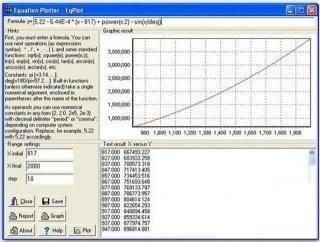
How to work with the program.
1. First, you must enter a formula.
You can use next operations (as expression syntax):
You can use next operations (as expression syntax):
Operators: + - * / and ( ) [parentheses]
Built-in Functions... [Unless otherwise indicated, all functions take a single numeric argument, enclosed in parentheses after the name of the function]
Algebraic: Abs, Square, Sqrt, Power(x;z) [= x raised to power of z; Use semicolor as the list-separator]
Transcendental: Exp, Ln [natural], LogBase10, LogBase2, LogBaseN(Base;x)
Trigonometric: Sin, Cos, Tan, Cot, Sec, Csc
Other Trig: ArcSin, ArcCos, ArcTan, ArcCot, ArcSec, ArcCsc, Coversine, Exsecans, Haversine, Versine
Hyperbolic: SinH, CosH, TanH, CotH, SecH, CscH
Other Hyp: ArcSinH, ArcCosH, ArcTanH, ArcCotH, ArcSecH, ArcCscH
Constants:{Mathematical constants}
Pi [= 3.1415926535897932384626433832795] {Pi}
PiOn2 [= 1.5707963267948966192313216916398] {Pi / 2}
PiOn3 [= 1.0471975511965977461542144610932] { Pi / 3}
PiOn4 [= 0.78539816339744830961566084581988] {Pi / 4}
Deg [= 57,295779513082320876798154814114] {180 / Pi}
Bernstein [= 0.2801694990238691330364364912307] {Bernstein constant}
Cbrt2 [= 1.2599210498948731647672106072782] {CubeRoot(2)}
Cbrt3 [= 1.4422495703074083823216383107801] {CubeRoot(3)}
Cbrt10 [= 2.1544346900318837217592935665194] {CubeRoot(10)}
Cbrt100 [= 4.6415888336127788924100763509194] {CubeRoot(100)}
CbrtPi [= 1.4645918875615232630201425272638] {CubeRoot(PI)}
Catalan [= 0.9159655941772190150546035149324] {Catalan constant}
Sqrt2 [= 1.4142135623730950488016887242097] {Sqrt(2)}
Sqrt3 [= 1.7320508075688772935274463415059] {Sqrt(3)}
Sqrt5 [= 2.2360679774997896964091736687313] {Sqrt(5)}
Sqrt10 [= 3.1622776601683793319988935444327] {Sqrt(10)}
SqrtPi [= 1.7724538509055160272981674833411] {Sqrt(Pi)}
Sqrt2Pi [= 2.506628274631000502415765284811] {Sqrt(2 * Pi)}
TwoPi [= 6.283185307179586476925286766559] {2 * Pi}
ThreePi [= 9.4247779607693797153879301498385] {3 * Pi}
Ln2 [= 0.69314718055994530941723212145818] {Ln(2)}
Ln10 [= 2.3025850929940456840179914546844] {Ln(10)}
LnPi [= 1.1447298858494001741434273513531] {Ln(Pi)}
Log2 [= 0.30102999566398119521373889472449] {LogBase10(2)}
Log3 [= 0.47712125471966243729502790325512] {LogBase10(3)}
LogPi [= 0.4971498726941338543512682882909] {LogBase10(Pi)}
LogE [= 0.43429448190325182765112891891661] {LogBase10(NConst)}
NConst [= 2.7182818284590452353602874713527] {Natural constant; exp(1)}
hLn2Pi [= 0.91893853320467274178032973640562] {Ln(2*Pi)/2}
inv2Pi [= 0.159154943091895] {0.5 / Pi}
TwoToPower63 [= 9223372036854775808.0] {263}
GoldenMean [= 1.618033988749894848204586834365638] {GoldenMean}
EulerMascheroni [= 0.5772156649015328606065120900824] {Euler GAMMA}
Constants:{Certain physical constants expressed in SI units}
Amu [= 1.6606E-27] {Atomic mass unit constant (kg)}
Avog [= 6.0225E23] {Avogadro constant (mol-1)}
Boltz [= 1.3805E-23] {Boltzmann constant (J K-1)}
ECharge [= 1.602189E-19] {Electron charge (C)}
EMass [= 9.11E-31] {Electron mass (kg)}
EVolt [= 1.602E-14] {Electron volt (J)}
Farad [= 96500] {Faraday constant (C mol-1)}
Gas [= 8.314] {Gas constant (J mol-1 K-1)}
Neutron [= 1.6748E-27] {Neutron mass (kg)}
Planck [= 6.626E-34] {Planck constant (Js)}
Proton [= 1.6725E-27] {Proton mass (kg)}
Light [= 2.9979E8] {Speed of light (m s-1)}
Gravity [= 9.80665] {Gravitational acceleration (m s-2)}
Pressure [= 101325] {Normal atmospheric pressure (N m-2)}
Stefan [= 5.67032E-8] {Stefan-Boltzmann constant (W m-2 K-4)}
Bohr [= 5.2917706E-11] {Bohr radius (m)}
> Note: Function and constant names are not case-sensitive. For example, Exp is the same as EXP or exp. The variable, which is the letter "x", is also not case-sensitive.
> Note: Text after proper mathematical expression will be ignored by the compiler. You can use this feature to comment your equation set.
> Note: In particular, you cannot use ^ for exponentiation, you must use the Power function instead.
> Note: All angle parameters and results of trigonometric functions are in radians. For degrees, multiply or divide by the Deg variable.
For example: Sin(30/Deg) will return 0.5, and ArcTan(1)*Deg will return 45.
> Note: All the algebraic, trigonometric, hyperbolic and transcendental routines map directly to Intel 80387 FPU floating point machine instructions.
> Note: The program is a graphing application and cannot be used as a scientific calculator. Though you can plot XY graph for floating-point values between 2.225E-308 (2-1022) and 1.797E+308 (21024), you cannot multiply two positive constants together with resulting values greater than 4096 (212). It is so designed. Use the "scientific calculator - ScienCalc" application instead.
> Note: As operands you can use numeric constants in any form (2, 2.0, 2e5, 2e-3) with decimal delimiter "period" or "comma", depending on your computer system configuration.
Example of formula: (2.0e-3*x) + square(x) + power(x;3) + power(2.55;4) + logbaseN(4;6.25)
Thus! If your computer system configuration uses "comma" as decimal delimiter/separator, 2.55 in the above example must be 2,55
Example of formula: (2,0e-3*x) + square(x) + power(x;3) + power(2,55;4) + logbaseN(4;6,25)
2. MaxX, minX: These are the limits of the drawing.
3. Step: The smaller value it has, the more accurate drawing you get.
Direct Download from attached file